Processing Field Spectroscopy Data
Introduction to Tutorial
This session will take you through the basic steps of processing, correcting, and visualising data acquired from a field spectrometer. The tools discussed in this session can be used to read data collected using any of the 350 nm to 2500 nm full range field spectrometers provided by the facility
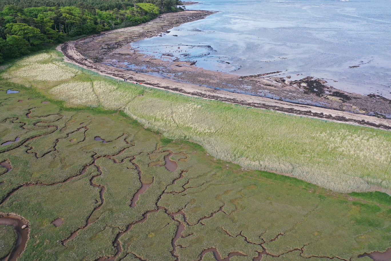
The data in this session was collected in May 2024 at a beach 40 km East of Edinburgh, United Kingdom (Tyninghame Links, 56.023, -2.592). Data was collected using a Spectra Vista Corporation HR-1024i full range field spectroradiometer in nadir viewing mode. Measurements were taken over a variety of different features, such as sand, dune grasses, and saltmarsh bogs.
Prior to this ground based data collection, multispectral UAV imagery was collected in March 2024. When collected in tandem, ground based and UAV measurements can work synergistically to produce powerful remote sensing products. We will develop a spectral library using the ground based hyperspectral data to help analyse the UAV imagery that we will look at later in today’s workshop.
Tutorial Steps
Part One – Creating a New Workbook, and Importing Modules
- Activate your field_spectroscopy environment you created in the last session, either via Anaconda Navigator, or via command prompt,
conda activate field_spectroscopy - Launch jupyterlab, via the Anaconda Navigator GUI or via the command prompt,
jupyter lab - In Jupyter Lab, navigate to the folder which you downloaded from the GitHub link provided in the last session.
- Open a new Notebook, by clicking New Launcher, then selecting Python 3 (ipykernel) under Notebook.
- In a new cell, copy and paste the following code, and then Run the cell using the play button in the ribbon, or by pressing
Ctrl + Enter
import os    #a module that allows us to "talk" with our operating system, necessary for handling paths, files and so on
from pathlib import Path #a more specific path handling module that allows us to quickly create path names
from specdal import Collection, Spectrum, read #We import our main package, specdal, and ask to only import certain key functions
import pandas as pd   #Pandas is a powerful module for the handling of data sets
from matplotlib import pyplot as plt   #matplotlib emulates the functions of MATLAB. Here, we tell matplotlib to only import one of it's functions, the pyplot function, and to import it with the identifier 'plt'
from matplotlib.pyplot import ylabel, xlabel, title, legend   #We go even further by asking pyplot to only import some of it's subfunctions
from scipy.signal import savgol_filter   #We will use this to smooth our data
import numpy as np #We require numpy for integration functions that will be used during convolution
import FieldSpecUtils as FSF
Part Two – Importing raw spectra files
In this first part of the session, we will use the SpecDAL module to help us import the raw spectral files collected (contained in the Data folder, in files with the .sig extension), assign to a pandas dataframe object, and – in the next parts – conduct basic corrections, such as interpolation, overlap matching, and jump correction.
- We will now use the SpecDAL package to read the .sig files found in our “Data” directory, and assign them to a collection of spectra which we can analyse and process further.
Copy and paste, then run, the following code into a new cell (from this point onwards, when new code is introduced, copy and paste it into a new cell below the last, and run):
Tyninghame = Collection(name='Tyninghame', directory ='Data') - Let’s now take a look at this spectra collection. First of all, let’s have a look at the header information for the first 3 spectra in our collection.
This not only prints the data itself (in the “measurements” category), but also the metadata associated with the file, such as GPS information.
print(type(Tyninghame.spectra)) for s in Tyninghame.spectra[0:3]: print(s) - You will notice that the spectra names follow a consistent naming structure – “[name]_[number]”. All name values correspond to a particular type of feature sampled. The subsequent number values are the samples acquired of that feature type. The feature types sampled at Tyninghame, and their relation to the name parameter, is as follows:
- Bog – spectra taken of vegetation that covered the saltmarsh bog to the West of the beach. The vegetation was a mix of rye grass, red fescue, and Sphagnum moss species.
- Driftwood – at various locations on the beach, driftwood features were found. These features can be of interest to ecological researchers.
- DrySand – dry sand, areas of the beach that were not under tide or inundated.
- DrySeaweed – beached seaweed that had dried.
- EBG – European Beach Grass, Ammophila arenaria, an important coastal dune grass species in Northern Europe. It has a thick root system which stabilizes dune systems.
- RG – perennial ryegrass, Lolium perenne
- SLG – sea lyme grass, Leymus arenarius, another important coastal dune species in Northern Europe.
- WetSand – inundated sand
- WetSeaweed – inundated seaweed
We can take a visual look at the data too:
Tyninghame.plot(figsize=(15, 6), legend = True, ylim=(0,1), xlim=(350, 2500))
xlabel("Wavelength (nm)")
ylabel("Relative Reflectance")
plt.legend(bbox_to_anchor=(1.05, 1), loc = "upper left")
plt.show()
Part Three – Grouping and Averaging Data
- It can be difficult to assess your data by viewing all spectra at once. We will group the data based on the name given to each type of feature using SpecDAL’s groupby function.
This groups data based on their file names, in this case the name before the “_” separator e.g. “bog”:
groups = Tyninghame.groupby(separator='_', indices=[0]) group_names = list(groups.keys()) print(group_names) - We can now limit our graph to show only one end member type, e.g. ‘SLG’:
groups['SLG'].plot(figsize=(15, 6), legend = True, ylim=(0,1), xlim=(350, 2500)) xlabel("Wavelength (nm)") ylabel("Relative Reflectance") plt.legend(bbox_to_anchor=(1.05, 1), loc = "upper left") plt.show()-
Question: - How would you modify the above code so that the graph displays the spectra for European Beach Grass?
Answer
Replace groups['SLG'] with groups['EBG']
-
Question: - How would you modify the above code so that the graph displays the spectra for European Beach Grass?
- We can then average each of these groups to produce a collection of means, called “means”:
means = Collection(name='means')
for group_key, group_collection in groups.items():
 means.append(group_collection.mean())
means.plot(title='Group means', figsize=(15, 6), ylim=(0, 1),xlim=(350, 2500))
xlabel("Wavelength (nm)")
ylabel("Relative Spectral Reflectance")
plt.show()
Part Four – Interpolation, overlap matching, and jump correction
- Look again at the print out for your data spectra, using data.head(10) function to print off the first 10 rows of data:
means.data.head(10) - For SVC instruments, the steps between the wavelengths correspond to the spectral resolution of the instrument, and are not resolved to 1 nm spacing.
In order to work with our data using standard routines, we would like to interpolate the reflectance measurements so that correspond to wavelengths with 1.0 nm spacing, a process called interpolation.
This can be done using SpecDAL as follows with the interpolate function:
means.interpolate(spacing=1, method='linear') means.data.head(10) - Take a look again at the 1000 nm region, and 1900 nm region, of the data:
means.plot(title='Group Means 1000nm Region', figsize=(15, 6), ylim=(0, 1),xlim=(950, 1050)) xlabel("Wavelength (nm)") ylabel("Relative Spectral Reflectance") plt.show() means.plot(title='Group Means 1900nm Region', figsize=(15, 6), ylim=(0, 1),xlim=(1850, 1950)) xlabel("Wavelength (nm)") ylabel("Relative Spectral Reflectance") plt.show() - A field spectrometer is designed so that it contains three different spectrometers, each covering a different range – a VNIR spectrometer to cover the visible to near infrared region (350 to 1000 nm);
a NIR spectrometer to cover the broader NIR region (1000 nm to 1900 nm); and a SWIR spectrometer to cover the shortwave infrared region (1900 to 2500 nm).
Each of these spectrometers overlaps in range, so that the final spectra has duplicated wavelength values.
We can resolve this issue by conducted overlap matching routines, which in SpecDAL, is provided by the stitch function:
means.stitch(method='mean') - If we inspect the regions again, we find that the duplication in the wavelength region has been removed, but that a small but sharp drop or increase in values persists at these regions, due to the different gain settings of the spectrometer.
To resolve this, we can conduct a “jump correction” using SpecDAL:
means.jump_correct(splices=[980, 1880], reference=0) - Plotting again shows that there is improvement in the 1000 nm region, but that the 1900 nm region is still noisy.
This is due to the presence of a strong water band absoprtion in this region. Later on, we will remove this region entirely, and interpolated between the extremes.
means.plot(title='Group means', figsize=(15, 6), ylim=(0, 1),xlim=(950, 1050))
xlabel("Wavelength (nm)")
ylabel("Relative Spectral Reflectance")
plt.show()
means.plot(title='Group means', figsize=(15, 6), ylim=(0, 1),xlim=(1850, 1950))
xlabel("Wavelength (nm)")
ylabel("Relative Spectral Reflectance")
plt.show()
Part Five – Relative vs Absolute Reflectance
Notice from our previous graphs that the y-axes are labelled “Relative Reflectance”. This is because these spectra were recorded relative to the reflectance of the white Spectralon panel. We take measurements relative to this panel to approximate the total irradiance coming from the light source (in this case, the Sun) and hitting the object you are interested in taking a spectral measurement of. Because the panel does not reflect 100% of the light that arrives on it’s surface in a completely uniform manner, we need to adjust our “Relative Reflectance” measurements using the panel’s known, laboratory calibrated reflectance to convert our field measurements to absolute reflectance.
We can derive the absolute reflectance then by multiplying our field measurements by the spectral reflectance of the panel for each wavelength. We can use this file to convert our measurements to absolute reflectance, pulling data from our calibration certificate, SRT_057_2023-0313.csv, which is located within the download folder. Note – we are creating new dataframes that will host the corrected values, but the original dataframe can be corrected without having to assign a new identifier.
As we only calibrate between the values of 350 to 2500 nm, we also top and tail the data to remove the regions 340 nm to 250 nm, and 2500 nm to 2510 nm, which have NaN values (the third line of code in the following cell).
reference_panel = pd.read_csv("SRT_057_2023-03013.csv", index_col = "Wavelength")
Absolute_Means = means.data.mul(reference_panel['Reflectance'], axis = 0)
Absolute_Means = Absolute_Means.iloc[10:2161]
Absolute_Means.head(10)
Part Six – Waterband removal over the 1780 nm to 1950 nm range, and smoothing across
As mentioned previously, the presence of a strong water band over the 1880 nm to 1950 nm range introduces noise and potentially spurious data to our spectra. As a best practice, we should remove regions in our spectra where water band absorption is likely to have introduced noise or error. Water bands also exist at other ranges across the 350 nm to 2500 nm spectrum, such as at 1300 nm and 1500 nm, but can often be ignored when dealing with ground spectroscopy data, where the atmospheric path length between spectrometer to the target is too small for such absorption to have an impact.
To conduct water band absorption removal, we isolate the specified region and replace all values with a NaN value. As many post processing workflows require that your spectral library contains no NaN or zero values, we will interpolate across this region.
Absolute_Means.iloc[1430:1630] = 1
Absolute_Means.replace(1,np.nan, inplace= True)
Absolute_Means.interpolate(method='linear', axis=0, inplace = True)
Absolute_Means.plot(title='Group means', figsize=(15, 6), ylim=(0, 1),xlim=(1700, 2200))
xlabel("Wavelength (nm)")
ylabel("Relative Spectral Reflectance")
plt.show()
To smooth the rest of our data, we will use the scipy pacakge .savgol_filter, which uses a Savitzky-Golay fitting technique to smooth 1D array data:
Absolute_Means_smoothed = pd.DataFrame(savgol_filter(Absolute_Means, 41, 2, axis=0),
                                       columns=Absolute_Means.columns,
                                       index=Absolute_Means.index)
Part Seven – Final processing stages for data
Let’s take a look at our final data output, where raw .sig files have been amalgamated into groups, averaged, interpolated, and converted to absolute reflectance:
Absolute_Means_smoothed.plot(title='Feature Means', figsize=(15, 6), ylim=(0, 1),xlim=(350, 2500))
xlabel("Wavelength (nm)")
ylabel("Absolute Spectral Reflectance")
plt.show()
We can now export this collection as a spectral library, that will be used in the next session for processing UAV imagery:
Absolute_Means_smoothed.to_csv(r'Tyninghame_Spectral_Lib_SNAP.csv', sep='\t', encoding='utf-8')
Wrapup
In this session, you’ve learned how to read full range field spectrometer data using Python, and conduct operations on that data to process it to the stage where it can be used for further remote sensing investigations. In the next session, we will go further, using the Absolute_Means_smoothed dataframe to generate remote sensing products like vegetation indices, and to convolve hyperspectral data to the mutlispectral bands of common in-orbit sensors.
Important For the next session, you will use Absolute_Means_smoothed dataframe. Please keep this frame active if progressing to the next session.